dcmri.Tissue#

class dcmri.Tissue(kinetics='HF', water_exchange='FF', sequence='SS', aif=None, ca=None, t=None, dt=1.0, free=None, **params)[source]#

Vascular-interstitial tissue.

This is the most common tissue type as found in for instance brain, cancer, lung, muscle, prostate, skin, and more. For more detail see Exchange tissues.

Parameters:

kinetics (str, optional) – Tracer-kinetic model. Possible values are ‘2CX’, ‘2CU’, ‘HF’, ‘HFU’, ‘NX’, ‘FX’, ‘WV’, ‘U’. Defaults to ‘HF’.
water_exchange (str, optional) – Water exchange regime. Any combination of two of the letters ‘F’, ‘N’, ‘R’ is allowed. Defaults to ‘FF’.
sequence (str, optional) – imaging sequence. Possible values are ‘SS’ and ‘SR’. Defaults to ‘SS’.
aif (array-like, optional) – Signal-time curve in the blood of the feeding artery. If aif is not provided, the arterial blood concentration is ca. Defaults to None.
ca (array-like, optional) – Blood concentration in the arterial input. ca is ignored if aif is provided, but is required otherwise. Defaults to None.
t (array-like, optional) – Time points of the arterial input function. If t is not provided, the temporal sampling is uniform with interval dt. Defaults to None.
dt (float, optional) – Time interval between values of the arterial input function. dt is ignored if t is provided. Defaults to 1.0.
free (dict, optional) – Dictionary with free parameters and their bounds. If not provided, a default set of free parameters is used. Defaults to None.
params (dict, optional) – values for the parameters of the tissue, specified as keyword parameters. Defaults are used for any that are not provided. See tables Tissue parameters and Parameter defaults for a list of tissue parameters and their default values.

See also

Liver, Kidney

Example

Fit an extended Tofts model to data:

>>> import dcmri as dc

Use fake_tissue to generate synthetic test data:

>>> time, aif, roi, gt = dc.fake_tissue(CNR=50)

Build a tissue and set the parameters to match the experimental conditions of the synthetic data:

>>> tissue = dc.Tissue(
...     aif = aif,
...     dt = time[1],
...     r1 = dc.relaxivity(3, 'blood','gadodiamide'),
...     TR = 0.005,
...     FA = 15,
...     n0 = 15,
... )

Train the tissue on the data:

>>> tissue.train(time, roi)

Print the optimized tissue parameters, their standard deviations and any derived parameters:

>>> tissue.print_params(round_to=2)

--------------------------------
Free parameters with their stdev
--------------------------------

Blood volume (vb): 0.03 (0.0) mL/cm3
Interstitial volume (vi): 0.2 (0.01) mL/cm3
Permeability-surface area product (PS): 0.0 (0.0) mL/sec/cm3

----------------------------
Fixed and derived parameters
----------------------------

Tissue Hematocrit (H): 0.45
Plasma volume (vp): 0.02 mL/cm3
Interstitial mean transit time (Ti): 71.01 sec
B1-corrected Flip Angle (FAcorr): 15 deg

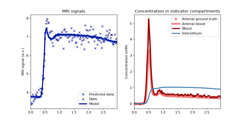
Plot the fit to the data and the reconstructed concentrations, using the noise-free ground truth as reference:

>>> tissue.plot(time, roi, ref=gt)

(Source code, png, hires.png, pdf)

Notes

Table Tissue parameters lists the parameters that are relevant in each regime. Alternatively, you can use dcmri.Tissue.info to print them out.

Table Parameter defaults list all possible parameters and their default settings.

**Tissue parameters**#
Parameters	When to use	Further detail
n0	Always	For estimating baseline signal
r1, R10	Always	Relaxation model parameters
R10a, B1corr_a	When aif is provided	Relaxation model parameters, Sequence parameters
S0, FA, TR, TS, B1corr	Always	Sequence parameters
TP, TC	If sequence is ‘SR’	Sequence parameters
Fb, PS, Ktrans, vb, H, vi, ve, vc, PSe, PSc.	Depends on kinetics and water_exchange	Parameters by configuration

**Parameter defaults**#
Parameter	Type	Value	Bounds	Free/Fixed
r1	Relaxation	5000.0	[0, inf]	Fixed
R10	Relaxation	0.7	[0, inf]	Fixed
R10a	Relaxation	0.7	[0, inf]	Fixed
B1corr	Sequence	1	[0, inf]	Fixed
B1corr_a	Sequence	1	[0, inf]	Fixed
FA	Sequence	15	[0, inf]	Fixed
S0	Sequence	1	[0, inf]	Fixed
TC	Sequence	0.1	[0, inf]	Fixed
TP	Sequence	0	[0, inf]	Fixed
TR	Sequence	0.005	[0, inf]	Fixed
TS	Sequence	0	[0, inf]	Fixed
H	Kinetic	0.45	[0, 1]	Fixed
Fb	Kinetic	0.01	[0, inf]	Free
Ktrans	Kinetic	0.002	[0, inf]	Free
PS	Kinetic	0.003	[0, inf]	Free
PSc	Kinetic	0.03	[0, inf]	Free
PSe	Kinetic	0.03	[0, inf]	Free
vb	Kinetic	0.1	[0, 1]	Free
vc	Kinetic	0.4	[0, 1]	Free
ve	Kinetic	0.355	[0, 1]	Free
vi	Kinetic	0.5	[0, 1]	Free

Methods

`conc`([sum])	Return the tissue concentration
`cost`(time, signal[, metric])	Return the goodness-of-fit
`export_params`()	Return model parameters with their descriptions
`info`()	Print detailed information about the tissue
`load`([file, path, filename])	Load the saved state of the model
`magnetization`()	Pseudocontinuous magnetization
`params`(*args[, round_to])	Return the parameter values
`plot`([time, signal, xlim, ref, fname, show])	Plot the model fit against data.
`predict`(time)	Predict the data at specific time points
`print_params`([round_to])	Print the model parameters and their uncertainties
`relax`()	Compartmental relaxation rates, volume fractions and water-permeability matrix.
`save`([file, path, filename])	Save the current state of the model
`set_free`([pop])	Set the free model parameters.
`signal`()	Pseudocontinuous signal
`time`()	Return an array of time points
`train`(time, signal[, method])	Train the free parameters

conc(sum=True)[source]#

Return the tissue concentration

Parameters:: sum (bool, optional) – If True, returns the total concentrations. Else returns the concentration in the individual compartments. Defaults to True.
Returns:: Concentration in M
Return type:: np.ndarray

Example

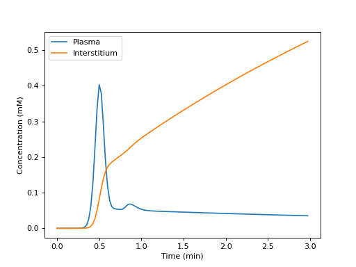
Build a tissue, and plot the tissue concentrations in each compartment:

>>> import dcmri as dc
>>> import matplotlib.pyplot as plt

>>> t, aif, _ = dc.fake_aif()
>>> tissue = dc.Tissue('HFU', 'RR', aif=aif, t=t)
>>> C = tissue.conc(sum=False)

>>> _ = plt.figure()
>>> _ = plt.plot(t/60, 1e3*C[0,:], label='Plasma')
>>> _ = plt.plot(t/60, 1e3*C[1,:], label='Interstitium')
>>> _ = plt.xlabel('Time (min)')
>>> _ = plt.ylabel('Concentration (mM)')
>>> _ = plt.legend()
>>> _ = plt.show()

(Source code, png, hires.png, pdf)

cost(time, signal, metric='NRMS') → float[source]#

Return the goodness-of-fit

Parameters:

time (array-like) – Array with time points.
signal (array-like) – Array with measured signals for each element of time.
metric (str, optional) – Which metric to use. Possible metrics are ‘RMS’ (Root-mean-square); ‘NRMS’ (Normalized root-mean-square); ‘AIC’ (Akaike information criterion); ‘cAIC’ (Corrected Akaike information criterion for small models); ‘BIC’ (Bayesian information criterion). Defaults to ‘NRMS’.

Returns:

goodness of fit.

Return type:

float

Example

Generate a fake dataset, build two tissues and use the Akaike Information Criterion to decide which configuration is most consistent with the data.

>>> import dcmri as dc
>>> t, aif, roi, _ = dc.fake_tissue()

>>> tissue1 = dc.Tissue('2CX','FF', t=t, aif=aif).train(t, roi)
>>> tissue2 = dc.Tissue('HFU','RR', t=t, aif=aif).train(t, roi)

>>> tissue1.cost(t, roi, 'AIC')
np.float64(-967.4477371121604)

>>> tissue2.cost(t, roi, 'AIC')
np.float64(-375.7766916566553)

tissue1 achieves the lowest cost and is therefore the optimal configuration according to the Akaike Information Criterion.

export_params()[source]#

Return model parameters with their descriptions

Returns:: Dictionary with one item for each model parameter. The key is the parameter symbol (short name), and the value is a 4-element list with [parameter name, value, unit, sdev].
Return type:: dict

Example

Train a tissue on synthetic data and print the blood volume after training:

>>> import dcmri as dc
>>> t, aif, roi, _ = dc.fake_tissue()
>>> tissue = dc.Tissue('HF','RR', t=t, aif=aif).train(t, roi)
>>> pars = tissue.export_params()
>>> pars['vb']
['Blood volume', np.float64(0.05735355675475683), 'mL/cm3', np.float64(0.016039245654090793)]

info()[source]#

Print detailed information about the tissue

Example

List all parameters of a default tissue:

>>> import dcmri as dc
>>> tissue = dc.Tissue()
>>> tissue.info()
-------------
Configuration
-------------
Kinetics: HF
Water exchange regime: FF
Imaging sequence: SS
----------
Parameters
----------
r1
--> Full name: Contrast agent relaxivity
--> Units: Hz/M
--> Initial value: 5000.0
--> Current value: 5000.0
--> Free parameter: No
--> Bounds: [0, inf]
R10a
--> Full name: Arterial precontrast R1
--> Units: Hz
--> Initial value: 0.7
--> Current value: 0.7
--> Free parameter: No
--> Bounds: [0, inf]
B1corr_a
--> Full name: Arterial B1-correction factor
--> Units:
--> Initial value: 1
--> Current value: 1
--> Free parameter: No
--> Bounds: [0, inf]
S0
--> Full name: Signal scaling factor
--> Units: a.u.
--> Initial value: 1.0
--> Current value: 1.0
--> Free parameter: No
--> Bounds: [0, inf]
B1corr
--> Full name: Tissue B1-correction factor
--> Units:
--> Initial value: 1
--> Current value: 1
--> Free parameter: No
--> Bounds: [0, inf]
FA
--> Full name: Flip angle
--> Units: deg
--> Initial value: 15
--> Current value: 15
--> Free parameter: No
--> Bounds: [0, inf]
TR
--> Full name: Repetition time
--> Units: sec
--> Initial value: 0.005
--> Current value: 0.005
--> Free parameter: No
--> Bounds: [0, inf]
TS
--> Full name: Sampling time
--> Units: sec
--> Initial value: 0
--> Current value: 0
--> Free parameter: No
--> Bounds: [0, inf]
H
--> Full name: Tissue Hematocrit
--> Units:
--> Initial value: 0.45
--> Current value: 0.45
--> Free parameter: No
--> Bounds: [0.001, 0.999]
vb
--> Full name: Blood volume
--> Units: mL/cm3
--> Initial value: 0.1
--> Current value: 0.1
--> Free parameter: Yes
--> Bounds: [0.001, 0.999]
vi
--> Full name: Interstitial volume
--> Units: mL/cm3
--> Initial value: 0.3
--> Current value: 0.3
--> Free parameter: Yes
--> Bounds: [0.001, 0.999]
PS
--> Full name: Permeability-surface area product
--> Units: mL/sec/cm3
--> Initial value: 0.003
--> Current value: 0.003
--> Free parameter: Yes
--> Bounds: [0, inf]
R10
--> Full name: Tissue precontrast R1
--> Units: Hz
--> Initial value: 0.7
--> Current value: 0.7
--> Free parameter: No
--> Bounds: [0, inf]
n0
--> Full name: Number of precontrast acquisitions
--> Units:
--> Initial value: 1
--> Current value: 1
--> Free parameter: No

load(file=None, path=None, filename='Model')#

Load the saved state of the model

Parameters:

file (str, optional) – complete path of the file. If this is not provided, a file is constructure from path and filename variables. Defaults to None.
path (str, optional) – path to store the state if file is not provided. Thos variable is ignored if file is provided. Defaults to current working directory.
filename (str, optional) – filename to store the state if file is not provided. If no extension is included, the extension ‘.pkl’ is automatically added. This variable is ignored if file is provided. Defaults to ‘Model’.

Returns:

class instance

Return type:

dict

magnetization() → ndarray[source]#

Pseudocontinuous magnetization

Returns:: the magnetization as a 1D array.
Return type:: np.ndarray

params(*args, round_to=None)[source]#

Return the parameter values

Parameters:

args (tuple) – parameters to get
round_to (int, optional) – Round to how many digits. If this is not provided, the values are not rounded. Defaults to None.

Returns:

values of parameter values, or a scalar value if only one parameter is required.

Return type:

list or float

Example

Train a tissue on synthetic data and print the compartment volumes:

>>> import dcmri as dc
>>> t, aif, roi, _ = dc.fake_tissue()
>>> tissue = dc.Tissue('HF','RR', t=t, aif=aif).train(t, roi)
>>> tissue.params('vp', 'vi', round_to=2)
[np.float64(0.03), np.float64(0.24)]

plot(time=None, signal=None, xlim=None, ref=None, fname=None, show=True)[source]#

Plot the model fit against data.

Parameters:

time (array-like, optional) – Array with time points.
signal (array-like, optional) – Array with measured signals for each element of time.
xlim (array_like, optional) – 2-element array with lower and upper boundaries of the x-axis. Defaults to None.
ref (tuple, optional) – Tuple of optional test data in the form (x,y), where x is an array with x-values and y is an array with y-values. Defaults to None.
fname (path, optional) – Filepath to save the image. If no value is provided, the image is not saved. Defaults to None.
show (bool, optional) – If True, the plot is shown. Defaults to True.

predict(time: ndarray) → ndarray[source]#

Predict the data at specific time points

Parameters:: time (array-like) – Array of time points.
Returns:: Array of predicted data for each element of time.
Return type:: np.ndarray

print_params(round_to=None)[source]#

Print the model parameters and their uncertainties

Parameters:: round_to (int, optional) – Round to how many digits. If this is not provided, the values are not rounded. Defaults to None.

Example

Train a tissue on synthetic data and print the parameters:

>>> import dcmri as dc
>>> t, aif, roi, _ = dc.fake_tissue()
>>> tissue = dc.Tissue('HF','RR', t=t, aif=aif).train(t, roi)
>>> tissue.print_params(round_to=2)

--------------------------------
Free parameters with their stdev
--------------------------------

Transendothelial water PS (PSe): 0.0 (0.22) mL/sec/cm3
Transcytolemmal water PS (PSc): 0.0 (1.39) mL/sec/cm3
Blood volume (vb): 0.06 (0.02) mL/cm3
Interstitial volume (vi): 0.24 (0.07) mL/cm3
Permeability-surface area product (PS): 0.0 (0.0) mL/sec/cm3

----------------------------
Fixed and derived parameters
----------------------------

Tissue Hematocrit (H): 0.45
Plasma volume (vp): 0.03 mL/cm3
Interstitial mean transit time (Ti): 83.27 sec
Intracellular water mean transit time (Twc): 1.3232576345772858e+16 sec
Interstitial water mean transit time (Twi): 186652627701867.1 sec
Intravascular water mean transit time (Twb): 47283940807705.62 sec
B1-corrected Flip Angle (FAcorr): 15 deg

relax()[source]#

Compartmental relaxation rates, volume fractions and water-permeability matrix.

tuple: relaxation rates of tissue compartments and their volumes.

R1 (numpy.ndarray): in the fast water exchange limit, the relaxation rates are a 1D array. In all other situations, relaxation rates are a 2D-array with dimensions (k,n), where k is the number of compartments and n is the number of time points in ca.
v (numpy.ndarray or None): the volume fractions of the tissue compartments. Returns None in ‘FF’ regime.
Fw (numpy.ndarray or None): 2D array with water exchange rates between tissue compartments. Returns None in ‘FF’ regime.

Example

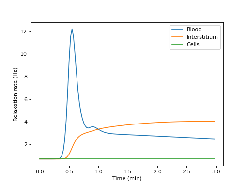
Build a tissue, print its compartmental volumes and water permeability matrix, and plot the free relaxation rates of each compartment:

>>> import dcmri as dc
>>> t, aif, _ = dc.fake_aif()
>>> tissue = dc.Tissue('2CX', 'RR', aif=aif, t=t)
>>> R1, v, Fw = tissue.relax()

>>> v
array([0.1, 0.3, 0.6])

>>> Fw
array([[0.  , 0.03, 0.  ],
       [0.03, 0.  , 0.03],
       [0.  , 0.03, 0.  ]])

>>> import matplotlib.pyplot as plt
>>> _ = plt.figure()
>>> _ = plt.plot(t/60, R1[0,:], label='Blood')
>>> _ = plt.plot(t/60, R1[1,:], label='Interstitium')
>>> _ = plt.plot(t/60, R1[2,:], label='Cells')
>>> _ = plt.xlabel('Time (min)')
>>> _ = plt.ylabel('Relaxation rate (Hz)')
>>> _ = plt.legend()
>>> plt.show()

(Source code, png, hires.png, pdf)

save(file=None, path=None, filename='Model')#

Save the current state of the model

Parameters:

file (str, optional) – complete path of the file. If this is not provided, a file is constructure from path and filename variables. Defaults to None.
path (str, optional) – path to store the state if file is not provided. Thos variable is ignored if file is provided. Defaults to current working directory.
filename (str, optional) – filename to store the state if file is not provided. If no extension is included, the extension ‘.pkl’ is automatically added. This variable is ignored if file is provided. Defaults to ‘Model’.

Returns:

class instance

Return type:

dict

set_free(pop=None, **kwargs)#

Set the free model parameters.

Parameters:

pop (str or list) – a single variable or a list of variables to remove from the list of free parameters.

Raises:

ValueError – if the pop argument contains a parameter that is not in the list of free parameters.
ValueError – If the parameter is not a model parameter, or bounds are not properly formatted.

signal() → ndarray[source]#

Pseudocontinuous signal

Returns:: the signal as a 1D array.
Return type:: np.ndarray

time()[source]#

Return an array of time points

Returns:: time points in seconds.
Return type:: np.ndarray

train(time, signal, method='NLLS', **kwargs)[source]#

Train the free parameters

Parameters:

time (array-like) – Array with time points.
signal (array-like) – Array with measured signals for each element of time.
method (str, optional) – Method to use for training. Currently the only option is ‘NNLS’ (Non-negative least squares). Default is ‘NNLS’.
kwargs – any keyword parameters accepted by the specified fit method. For ‘NNLS’ these are all parameters accepted by scipy.optimize.curve_fit, except for bounds.

Returns: