An exploration of water exchange effects

This tutorial will explore the effect of water exchange in a standard two-compartmental tissue using the models in dcmri.Tissue.

The three tissue compartments involved are the blood, interstitium and tissue cells. The water exchange effects refer to the transport of water across the barriers between them: transendothelial water exchange between blood and interstitium, and transcytolemmal water exchange between interstitium and tissue cells. The water exchange in the blood compartment between plasma and red blood cells is assumed to be in the fast exchange limit.

Water exchange across either of these two barriers can be in the fast-exchange limit (F), restricted (R), or there may be no water exchange at all (N). Since there are two barriers involved this leads to 3x3=9 possible water exchange regimes. dcmri.Tissue denotes these 9 regimes by a combination of the letters F, R and N: the frst letter refers to the water exchange across the endothelium, and the second to the water exchange across the cell wall. For instance, ‘FR’ means fast water exchange (F) across the endothelium, and restricted water exchange (R) across the cell wall.

For regimes with restricted water exchange, the rate of exchange is quantified by the permeability-surface area (PS) of water, a quantity in units of mL/sec/cm3. dcmri.Tissue uses the notation PSe for the transendothelial water PS and PSc for the transcytolemmal PS.

Simulation setup

We set up the simulation by importing the necessary packages and defining the constants that will be fixed throughout.

import matplotlib.pyplot as plt
import dcmri as dc

# Generate a synthetic AIF with default settings
t, aif, _ = dc.fake_aif(tacq=300)

# Save AIF and its properties in a dictionary
aif = {
    't': t,
    'aif': aif,
    'r1': dc.relaxivity(3, 'blood', 'gadodiamide'),
    'R10a': 1/dc.T1(3.0,'blood'),
}

The role of water exchange

To show how water exchange is relevant in DC-MRI analysis, it is insightful to first consider the extreme ends of the water exchange spectrum in some more detail: fast water exchange (F) and no water exchange (N).

Let’s first generate a tissue without water exchange across either barrier. We will use the more general model of restricted water exchange ‘RR’ and set the permeabilities to zero, as this then also plots the signals in individual compartments:

tissue_nn = dc.Tissue('2CX', 'RR', PSe=0, PSc=0, **aif)
tissue_nn.plot()

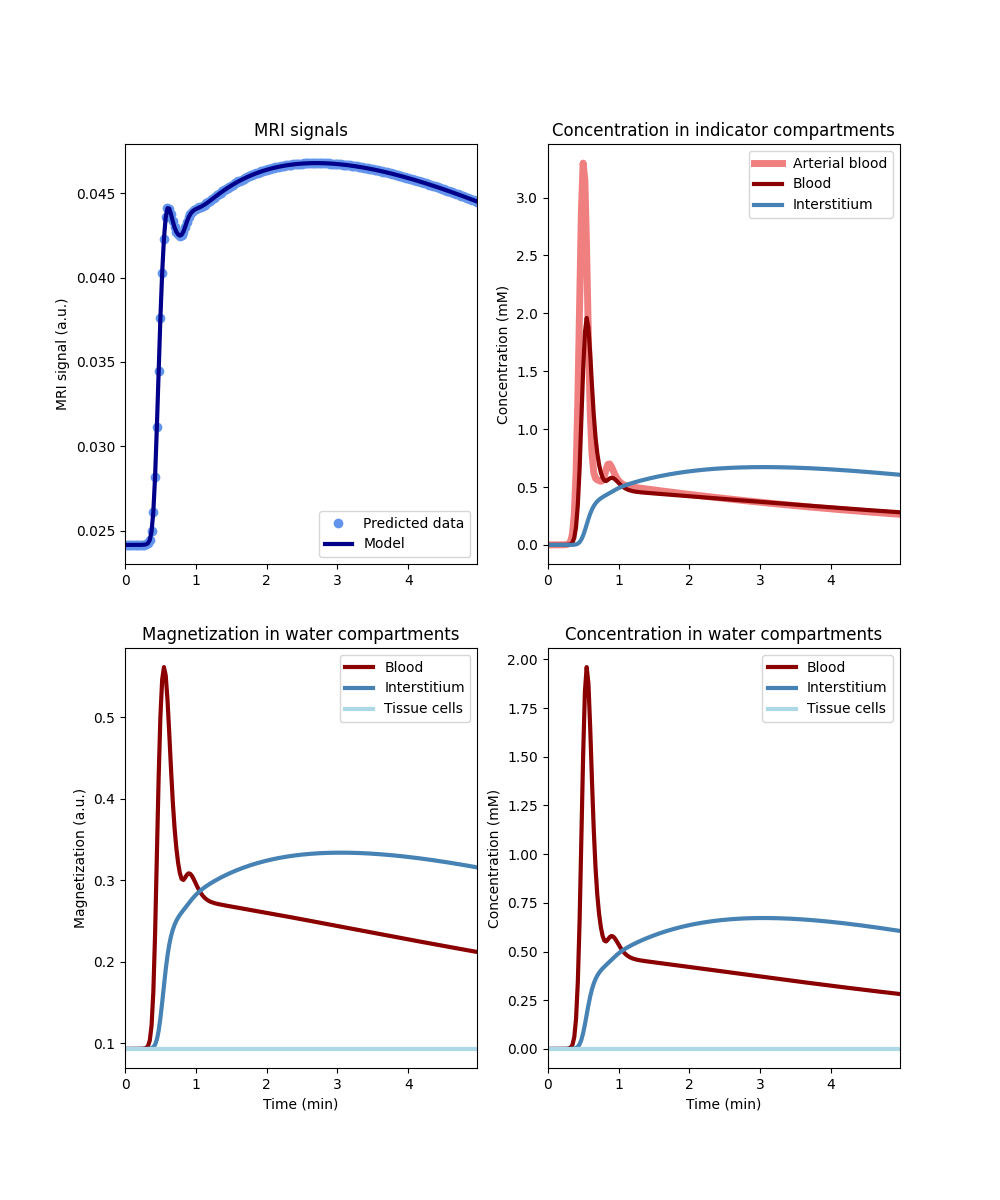
In this model the indicator and water occupy the same compartments, so the concentrations on the right are the same. The magnetization (bottom left) follows the profile of the indicator concentrations exactly: since magnetization cannot exchange, it cannot equilibrate and remains directly proportional to the concentration in the compartment. Notably, the magnetization in the tissue cells remains constant as no indicator can enter this compartment to modify it, and no magnetization can be transferred.

Now lets consider the opposite scenario of fast water exchange across both barriers (Note: we could use the FF model here, but for the purposes of this illustration it is more instructive to use RR with very high values for the water permeabilities):

tissue_ff = dc.Tissue('2CX','RR', PSe=1e3, PSc=1e3, **aif)
tissue_ff.plot()

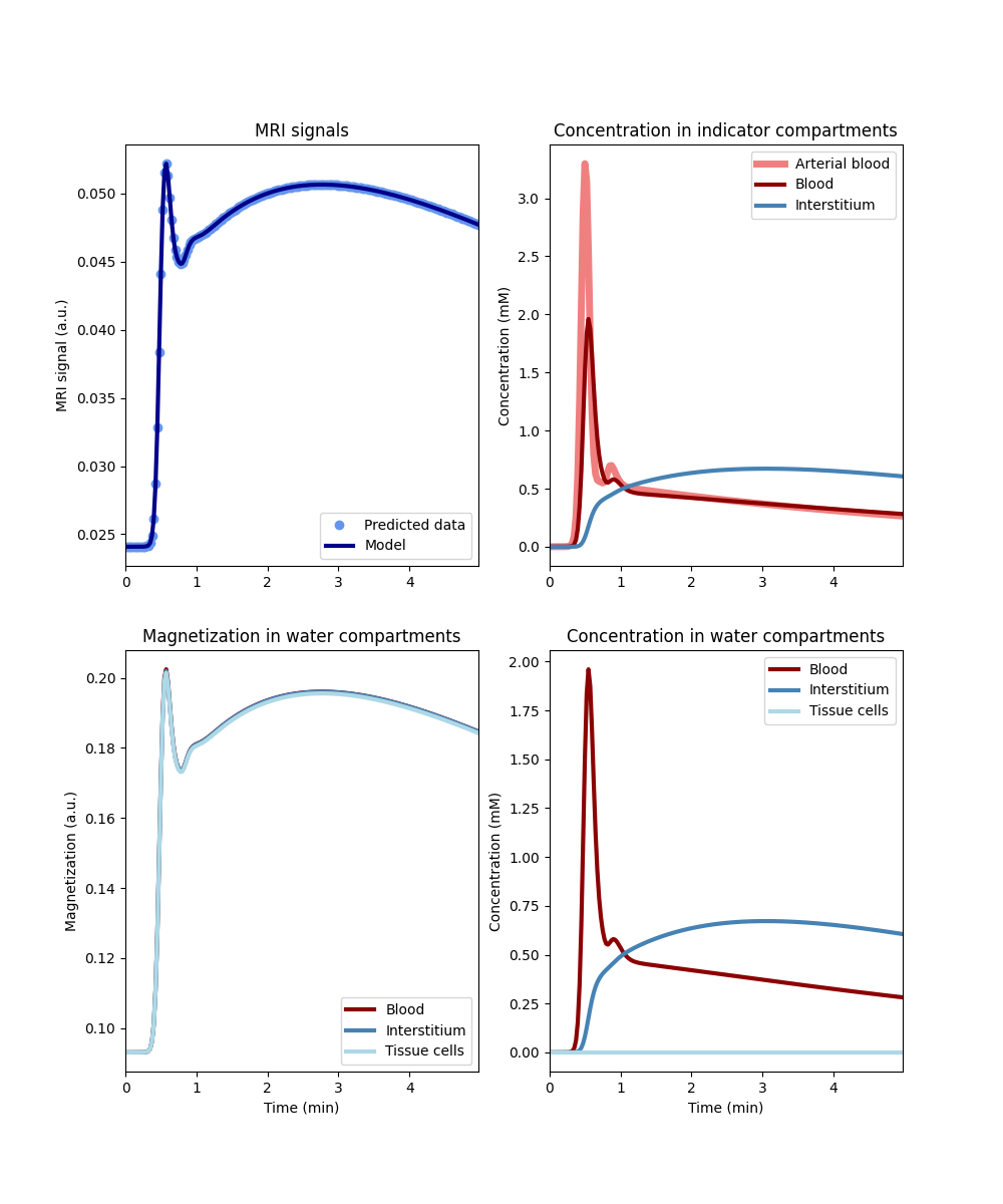
The indicator concentration in the tissue compartments is not affected by the level of water exchange (top and bottom right), but the magnetization in all 3 compartments is now effectively the same (bottom left). Even the tissue cells, which receive no indicator at all, show the same signal changes over time as the interstitium and blood compartments. This is because, with very high levels of water exchange, the magnetization between all 3 compartments mixes so rapidly that any differences are levelled out instantly. The tissue is well-mixed for water (and therefore water magnetization), although it is not well-mixed for indicator.

Now let’s consider the cases where one of the barriers is highly permeable for water, and the other is impermeable. First let’s look at the case of high transendothelial water exchange and no transcytolemmal water exchange:

tissue_fn = dc.Tissue('2CX','RR', PSe=1e3, PSc=0, **aif)
tissue_fn.plot()

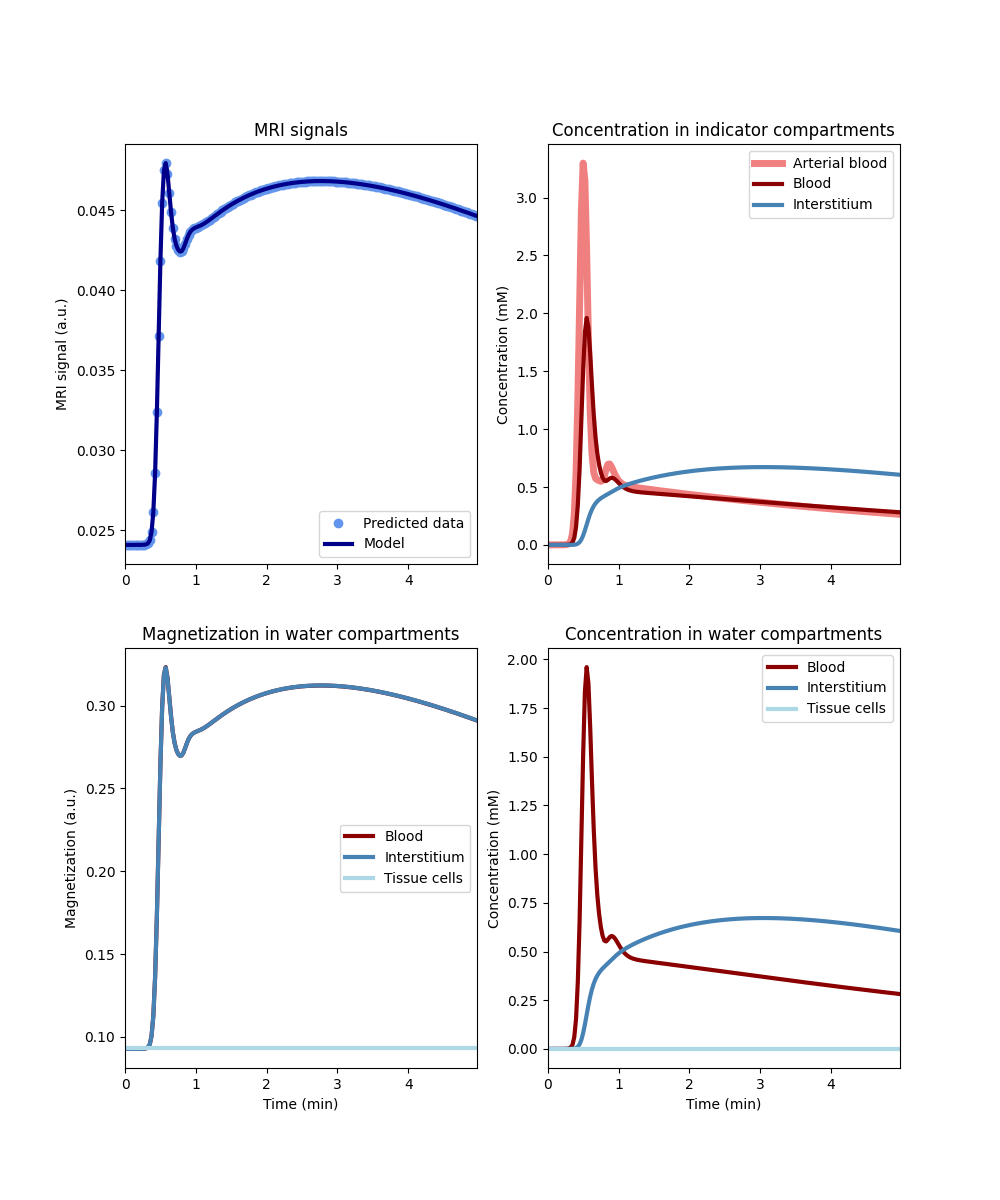
As expected, blood and interstitium have the same magnetization throughout and the magnetization of tissue cells is not altered at all. The opposite case is similar:

tissue_nf = dc.Tissue('2CX','RR', PSe=0, PSc=1e3, **aif)
tissue_nf.plot()

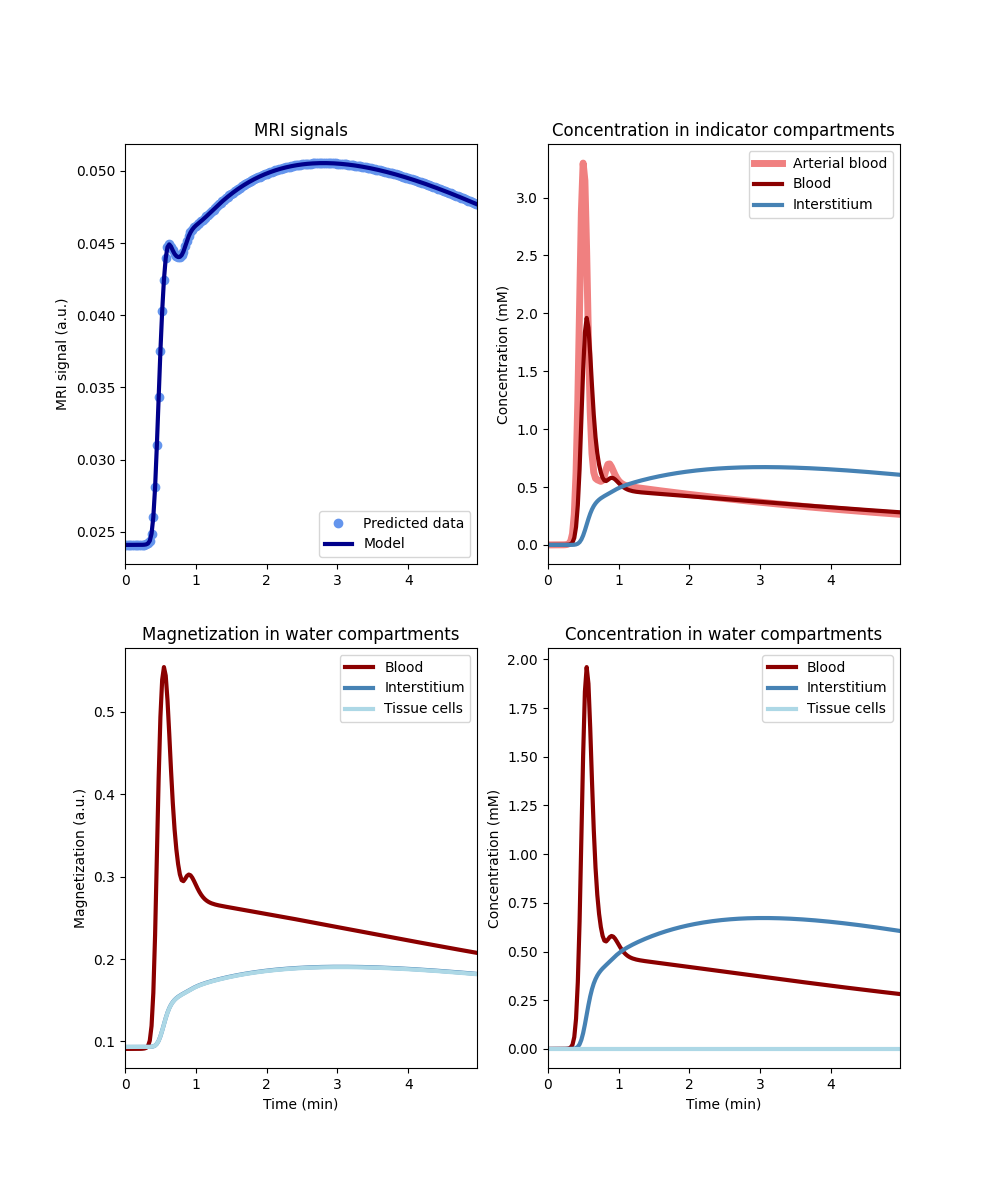
In this case the tissue cells recieve the same magnetization as the interstitium.

Water exchange effect on the MR signal

From a measurement perspective, the important question is to what extent water exchange across either barrier affects the measured signal, shown in the top left corner of the plots above.

To illustrate the signal differences in more detail, we plot signals in mixed exchange regimes against the extremes of fast and no exchange. For reference we also include a tissue with intermediate water exchange:

# Build a tissue in an intermediate water exchange regime
tissue_rr = dc.Tissue('2CX','RR', PSe=1, PSc=2, **aif)

# Generate signals in all regimes
signal_ff = tissue_ff.signal()
signal_nn = tissue_nn.signal()
signal_fn = tissue_fn.signal()
signal_nf = tissue_nf.signal()
signal_rr = tissue_rr.signal()

# Plot signals against extremes
fig, ax = plt.subplots(1,3,figsize=(15,5))

ax[0].set_title("""No transendothelial exchange \n
                Fast transcytolemmal exchange""")
ax[1].set_title("""Fast transendothelial exchange \n
                No transcytolemmal exchange""")
ax[2].set_title("""Restricted transendothelial exchange \n
                Restricted transcytolemmal exchange""")

ax[0].plot(t, signal_nf, 'r--', label='Mixed exchange')
ax[1].plot(t, signal_fn, 'r--', label='Mixed exchange')
ax[2].plot(t, signal_rr, 'r--', label='Restricted exchange')

for axis in ax:
    axis.plot(t, signal_ff, 'g-', label='Fast exchange')
    axis.plot(t, signal_nn, 'b-', label='No exchange')
    axis.set_xlabel('Time (sec)')
    axis.set_ylabel('Signal (a.u.)')
    axis.legend()

plt.show()

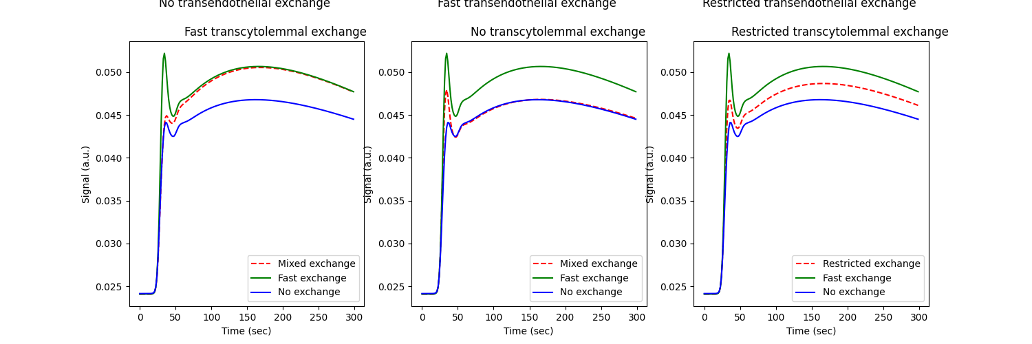
These figures show clearly that water exchange levels have a measureable effect on signals, and at all times lie between the extremes of no water exchange (blue) and fast water exchange (green).

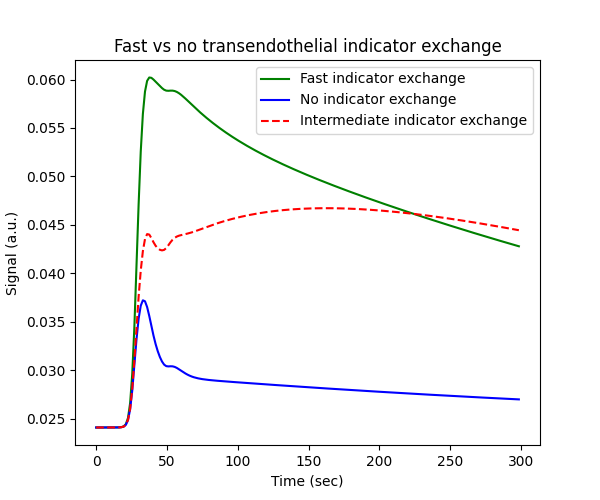
However, while the effect of water exchange is detectable, it is comparatively small considering the difference between the blue and green curves represent the extremes. By contrast, changing the exchange rate of the indicator between its extremes of no- and infinite indicator exchange has a more significant impact on the signal:

tissue_2cx = dc.Tissue('2CX','RR', **aif)
tissue_nx = dc.Tissue('2CX','RR', PS=0, **aif)
tissue_fx = dc.Tissue('2CX','RR', PS=1e3, **aif)

# Plot signals
fig, ax = plt.subplots(1,1,figsize=(6,5))

ax.set_title('Fast vs no transendothelial indicator exchange')
ax.plot(t, tissue_fx.signal(), 'g-', label='Fast indicator exchange')
ax.plot(t, tissue_nx.signal(), 'b-', label='No indicator exchange')
ax.plot(t, tissue_2cx.signal(), 'r--', label='Intermediate indicator exchange')
ax.set_xlabel('Time (sec)')
ax.set_ylabel('Signal (a.u.)')
ax.legend()

plt.show()

Water exchange bias

As shown above, water exchange is to some extent a second order effect compared to indicator exchange. Nevertheless, making inaccurate assumptions regarding the level of water exchange can lead to large biases in the other measured parameters.

One way to explore the scale of this water exchange bias is by training a tissue that has no water exchange (NN) using data generated by a tissue in fast water exchange:

# Train a NN tissue on the fast-exchange signal and plot results
tissue_nn = dc.Tissue('2CX', 'NN', **aif)
tissue_nn.train(t, signal_ff)
tissue_nn.plot(t, signal_ff)

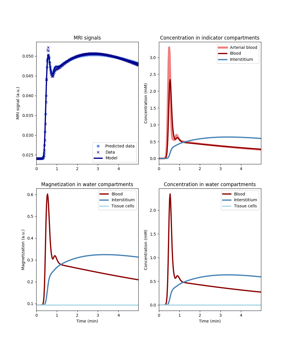
The plot shows that the no-exchange tissue predicts the data with high accuracy. However, the reconstructed magnetization is incorrect for fast exchange tissue, and the reconstructed parameters are severely biased:

truth = tissue_ff.params('vp','vi','Ktrans')
rec = tissue_nn.params('vp','vi','Ktrans')
print('vp error:', round(100*(rec[0]-truth[0])/truth[0],1), '%')
print('vi error:', round(100*(rec[1]-truth[1])/truth[1],1), '%')
print('Ktrans error:', round(100*(rec[2]-truth[2])/truth[2],1), '%')

vp error: 40.5 %
vi error: 16.9 %
Ktrans error: 0.9 %

Removing water exchange bias

Water exchange forms a dangerous source of measurement error because it cannot be detected by comparing the fit to the data. In ideal circumstances, it can be removed by generalizing the model to allow for any level of water exchange. Let’s try this and look at the results again:

# Train an RR tissue and plot again
tissue = dc.Tissue('2CX','RR', **aif)
tissue.train(t, signal_ff, xtol=1e-3)
tissue.plot(t, signal_ff)

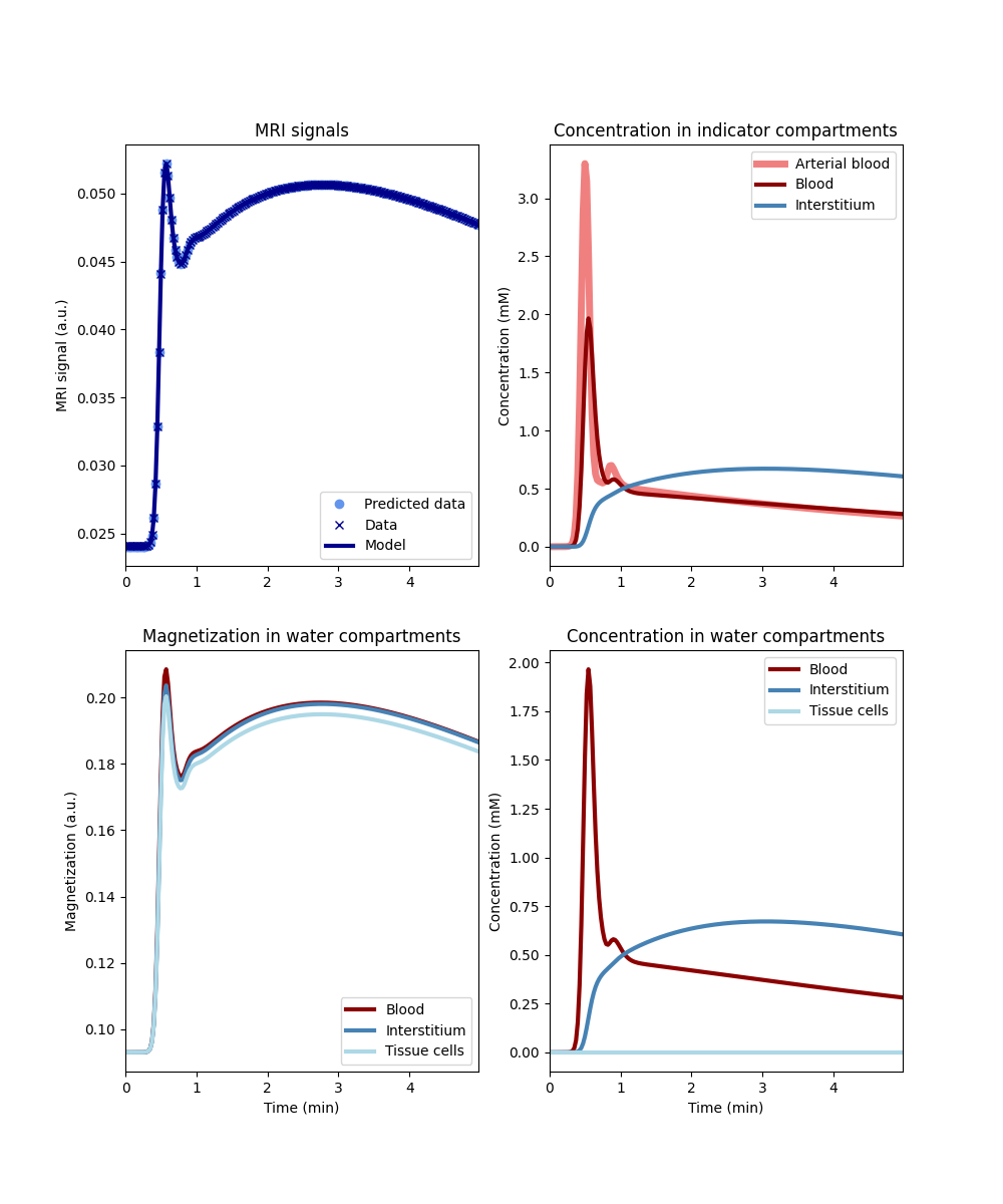
Plotting the results now show a practically perfect fit to the data, and the magnetization is close to the fast exchange limit. Also the measurements of the kinetic parameters are more accurate:

rec = tissue.params('vp','vi','Ktrans')
print('vp error:', round(100*(rec[0]-truth[0])/truth[0],1), '%')
print('vi error:', round(100*(rec[1]-truth[1])/-truth[1],1), '%')
print('Ktrans error:', round(100*(rec[2]-truth[2])/truth[2],1), '%')

vp error: 1.0 %
vi error: -0.8 %
Ktrans error: 0.7 %

As a bonus the water-exchange sensitive model also estimates the water permeability. While a numerical fit will not produce the accurate result of infinite water PS, this nevertheless produces values that correspond to extremely high levels of water exchange:

rec = tissue.params('PSe', 'PSc', round_to=0)
print('PSe:', rec[0], 'mL/sec/cm3')
print('PSc:', rec[1], 'mL/sec/cm3')

PSe: 106.0 mL/sec/cm3
PSc: 147.0 mL/sec/cm3

Handling water exchange

The above example suggests one strategy of removing water exchange bias, i.e. include water exchange rates as free parameters and get the added benefit of a water exchange measurement. However this may not always be the right approach. The data in this tutorial are noise-free, and therefore even very subtle structure can be exploited to estimate parameters. In noisy data this may not be the case, and one may well be forced to fix parameters that have a relatively small effect on the data in order to improve the precision in others.

This raises the question where any of the regimes of fast and zero water exchange offers a good approximation to real tissues. For this exercise we will assume values on the upper end of literature data. We plot the resulting signal against the extremes of fast and no exchange:

# Generate tissue
tissue = dc.Tissue('2CX', 'RR', PSe=0.05, PSc=1.5, **aif)
tissue_nn = dc.Tissue('2CX', 'NN', **aif)
tissue_ff = dc.Tissue('2CX', 'FF', **aif)

# Plot signals
fig, ax = plt.subplots(1,1,figsize=(6,5))

ax.set_title('Restricted water exchange against extremes')
ax.plot(t, tissue_ff.signal(), 'g-', label='Fast water exchange')
ax.plot(t, tissue_nn.signal(), 'b-', label='No water exchange')
ax.plot(t, tissue.signal(), 'r--', label='Restricted water exchange')
ax.set_xlabel('Time (sec)')
ax.set_ylabel('Signal (a.u.)')
ax.legend()

plt.show()

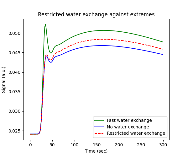
With these settings, the restricated water exchange signal is approximately intermediate between fast and no water exchange. Hence neither approximation appears particulare more accurate than the alternative.

However, the impact of water exchange also depends on the imaging sequence, such as the choice of flip angle. Hence these effects should be taken into account when optimizing the scan protocol. Water exchange sensitivity should be maximized for studies that aim to measure it, and minimized for studies where it is a confounder.