dcmri.conc_kidney

dcmri.conc_kidney(ca: ndarray, *params, t=None, dt=1.0, sum=True, kinetics='2CF', **kwargs) → ndarray

Concentration in kidney tissues.

Parameters:

• ca (array-like) – concentration in the arterial input.

• params (tuple) – free model parameters.

• t (array_like, optional) – the time points in sec of the input function ca. If t is not provided, the time points are assumed to be uniformly spaced with spacing dt. Defaults to None.

• dt (float, optional) – spacing in seconds between time points for uniformly spaced time points. This parameter is ignored if t is explicity provided. Defaults to 1.0.

• kinetics (str, optional) – Kinetics of the tissue, either ‘2CF’, ‘FN’ - see below for detail. Defaults to ‘2CF’.

• sum (bool, optional) – For two-compartment tissues, set to True to return the total tissue concentration. Defaults to True.

• kwargs (dict, optional) – any optional keyword parameters required by the kinetic model - see below for detail.

Returns:

If sum=True, this is a 1D array with the total concentration at each time point. If sum=False this is the concentration in each compartment, and at each time point, as a 2D array with dimensions (2,k), where k is the number of time points in ca. The concentration is returned in units of M.

Return type:

numpy.ndarray

Notes

Currently implemented kinetic models are:

• ‘2CF’: two-compartment filtration model. params = (Fp, Tp, Ft, Tt,)

• ‘FN’: free nephron model. params = (Fp, Tp, Ft, h, ).

The model parameters are:

• Fp (float, mL/sec/mL): Plasma flow.

• Tp (float, sec): plasma mean transit time.

• Ft (float, mL/sec/mL): tubular flow.

• Tt (float, sec): tubular mean transit time.

• hh (array-like, 1/sec): frequences of transit time histogram. The boundaries of the transit time bins can be provided as an array in a keyword parameter TT, which has to have one more element than h. If TT is not provided, the transit time bins are equally space in the range [0, tmax], where tmax is the largest acquisition time.

Example

Plot concentration in cortex and medulla for typical values:

>>> import matplotlib.pyplot as plt
>>> import numpy as np
>>> import dcmri as dc

Generate a population-average input function:

>>> t = np.arange(0, 300, 1.5)
>>> ca = dc.aif_parker(t, BAT=20)

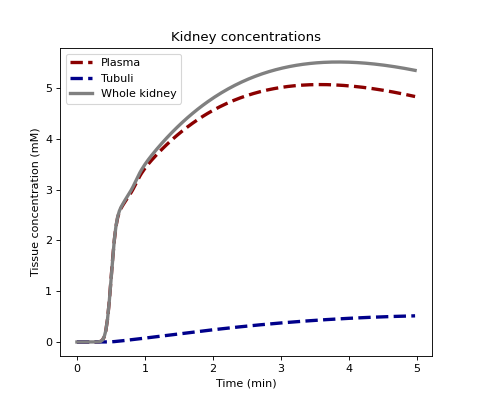
Define some parameters and generate plasma and tubular tissue concentrations with a 2-compartment filtration model:

>>> Fp, Tp, Ft, Tt = 0.05, 10, 0.01, 120
>>> C = dc.conc_kidney(ca, Fp, Tp, Ft, Tt, t=t, sum=False, kinetics='2CF')

Plot all concentrations:

>>> fig, ax = plt.subplots(1,1,figsize=(6,5))
>>> ax.set_title('Kidney concentrations')
>>> ax.plot(t/60, 1000*C[0,:], linestyle='--', linewidth=3.0, color='darkred', label='Plasma')
>>> ax.plot(t/60, 1000*C[1,:], linestyle='--', linewidth=3.0, color='darkblue', label='Tubuli')
>>> ax.plot(t/60, 1000*(C[0,:]+C[1,:]), linestyle='-', linewidth=3.0, color='grey', label='Whole kidney')
>>> ax.set_xlabel('Time (min)')
>>> ax.set_ylabel('Tissue concentration (mM)')
>>> ax.legend()
>>> plt.show()

(Source code, png, hires.png, pdf)

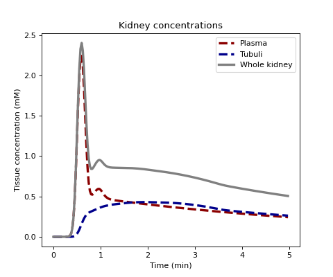
Use generate plasma and tubular tissue concentrations using the free nephron model for comparison. We assume 4 transit time bins with the following boundaries (in units of seconds):

>>> TT = [0, 15, 30, 60, 120]

with longest transit times most likely (note the frequences to not have to add up to 1):

>>> h = [1, 2, 3, 4]
>>> C = dc.conc_kidney(ca, Fp, Tp, Ft, h, t=t, sum=False, kinetics='FN', TT=TT)

Plot all concentrations:

>>> fig, ax = plt.subplots(1,1,figsize=(6,5))
>>> ax.set_title('Kidney concentrations')
>>> ax.plot(t/60, 1000*C[0,:], linestyle='--', linewidth=3.0, color='darkred', label='Plasma')
>>> ax.plot(t/60, 1000*C[1,:], linestyle='--', linewidth=3.0, color='darkblue', label='Tubuli')
>>> ax.plot(t/60, 1000*(C[0,:]+C[1,:]), linestyle='-', linewidth=3.0, color='grey', label='Whole kidney')
>>> ax.set_xlabel('Time (min)')
>>> ax.set_ylabel('Tissue concentration (mM)')
>>> ax.legend()
>>> plt.show()

(png, hires.png, pdf)