dcmri.conc_tissue#
- dcmri.conc_tissue(ca: ndarray, t=None, dt=1.0, kinetics='2CX', sum=True, **params) ndarray[source]#
Tissue concentration in a 2-site exchange tissue.
- Parameters:
ca (array-like) – concentration in the arterial input.
t (array_like, optional) – the time points of the input function ca. If t is not provided, the time points are assumed to be uniformly spaced with spacing dt. Defaults to None.
dt (float, optional) – spacing in seconds between time points for uniformly spaced time points. This parameter is ignored if t is provided. Defaults to 1.0.
kinetics (str, optional) – Tracer-kinetic model. Possible values are ‘2CX’, ‘2CU’, ‘HF’, ‘HFU’, ‘NX’, ‘FX’, ‘WV’, ‘U’ (see table Kinetic models for detail). Defaults to ‘2CX’.
sum (bool, optional) – For two-compartment tissues, set to True to return the total tissue concentration, and False to return the concentrations in the compartments separately. In one-compartment tissues this keyword has no effect. Defaults to True.
params (dict) – free model parameters provided as keyword arguments. Possible parameters depend on kinetics as detailed in Table Kinetic models.
- Returns:
- concentration
If sum=True, or the tissue is one-compartmental, this is a 1D array with the total concentration at each time point. If sum=False this is the concentration in each compartment, and at each time point, as a 2D array with dimensions (2,k), where k is the number of time points in ca.
- Return type:
- Raises:
ValueError – if values are not provided for one or more of the model parameters.
Example
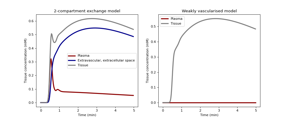
We plot the concentrations of 2CX and WV models with the same values for the shared tissue parameters.
Start by importing the packages:
>>> import matplotlib.pyplot as plt
>>> import numpy as np
>>> import dcmri as dc
Generate a population-average input function:
>>> t = np.arange(0, 300, 1.5)
>>> ca = dc.aif_parker(t, BAT=20)
Define some tissue parameters:
>>> p2x = {'H': 0.5, 'vb':0.1, 'vi':0.4, 'Fb':0.02, 'PS':0.005}
>>> pwv = {'H': 0.5, 'vi':0.4, 'Ktrans':0.005*0.01/(0.005+0.01)}
Generate plasma and extravascular tissue concentrations with the 2CX and WV models:
>>> C2x = dc.conc_tissue(ca, t=t, sum=False, kinetics='2CX', **p2x)
>>> Cwv = dc.conc_tissue(ca, t=t, kinetics='WV', **pwv)
Compare them in a plot:
>>> fig, (ax0, ax1) = plt.subplots(1,2,figsize=(12,5))
Plot 2CX results in the left panel:
>>> ax0.set_title('2-compartment exchange model')
>>> ax0.plot(t/60, 1000*C2x[0,:], linestyle='-', linewidth=3.0,
>>>          color='darkred', label='Plasma')
>>> ax0.plot(t/60, 1000*C2x[1,:], linestyle='-', linewidth=3.0,
>>>          color='darkblue',
>>>          label='Extravascular, extracellular space')
>>> ax0.plot(t/60, 1000*(C2x[0,:]+C2x[1,:]), linestyle='-',
>>>          linewidth=3.0, color='grey', label='Tissue')
>>> ax0.set_xlabel('Time (min)')
>>> ax0.set_ylabel('Tissue concentration (mM)')
>>> ax0.legend()
Plot WV results in the right panel:
>>> ax1.set_title('Weakly vascularised model')
>>> ax1.plot(t/60, Cwv*0, linestyle='-', linewidth=3.0,
>>>          color='darkred', label='Plasma')
>>> ax1.plot(t/60, 1000*Cwv, linestyle='-',
>>>          linewidth=3.0, color='grey', label='Tissue')
>>> ax1.set_xlabel('Time (min)')
>>> ax1.set_ylabel('Tissue concentration (mM)')
>>> ax1.legend()
>>> plt.show()
(
Source code,png,hires.png,pdf)
