A comparison of convolution functions

Convolution is a key operation in any application of pharmacokinetic analysis. The reason for this central role is that the solution of a linear and stationary system can always be written as a convolution. dcmri includes functions that perform convolution in the most general context, but also includes solutions that are optimized for common special cases.

This tutorial illustrates the use of these functions and compares their performance against other implementations.

Setup

Import the necessary packages

import time
import numpy as np
from scipy.stats import norm
import matplotlib.pyplot as plt
import dcmri as dc

Convolving any two functions

There are different definitions possible for the convolution product, and they are not necessarily interchangeable. We illustrate this here by convolving two functions with conv and comparing the result to a naive application of numpy.convolve. For the purposes of this illustration we will convolve normalized gaussian distributions f(t) and h(t):

# Generate some gaussian data
t = np.linspace(0, 100, 50)
f = norm.pdf(t, 30, 5)
h = norm.pdf(t, 60, 10)

# Convolve them in two different ways:
g = dc.conv(h, f, t)
g1 = np.convolve(h, f, mode='same')

# Show the data and their convolutions
plt.plot(t, f, 'r-', label='f(t)')
plt.plot(t, h, 'b-', label='h(t)')
plt.plot(t, g, 'k-', label='dcmri.conv')
plt.plot(g1, 'k:', label='numpy.convolve')
plt.title('Convolution of two gaussian distributions')
plt.legend()
plt.show()

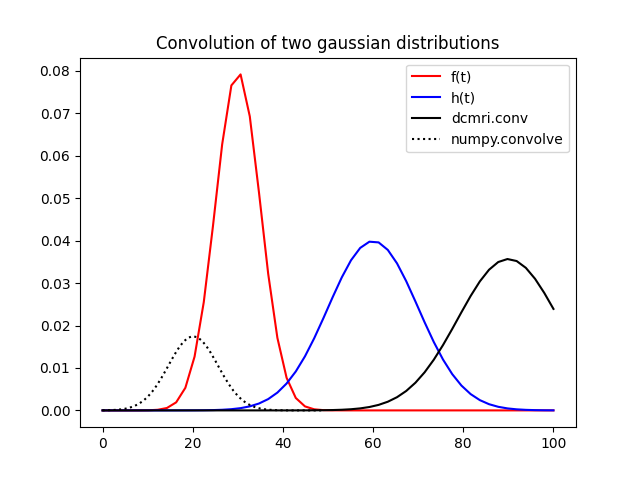
While there is clearly some relation between both results, they are not in any way similar. The convolve result is shifted compared to conv and has a lower amplitude. This shows that caution is needed when applying convolution formulae from different libraries in a tracer-kinetic setting.

Convolution with an exponential

The generic function conv applies to any two functions, but is uneccesarily slow in special cases where the functional form of the factors is known. An example is the case where one of the factors is an exponential function - a very common scenario in pharmacokinetics. In that case the function expconv can be used:

# Convolve the Gaussian with an exponential explicitly:
Tf = 20
f = np.exp(-t/Tf)/Tf
g0 = dc.conv(h, f, t)

# Now convolve the same data again using the expconv function:
g1 = dc.expconv(h, Tf, t)

# Compare the two results on the same plot:
plt.plot(t, f, 'r-', label='f(t)')
plt.plot(t, h, 'b-', label='h(t)')
plt.plot(t, g0, label='conv()', linewidth=6, color='lightgray', linestyle='-')
plt.plot(t, g1, 'k-', label='expconv()')
plt.title('Comparison of conv() and expconv()')
plt.legend()
plt.show()

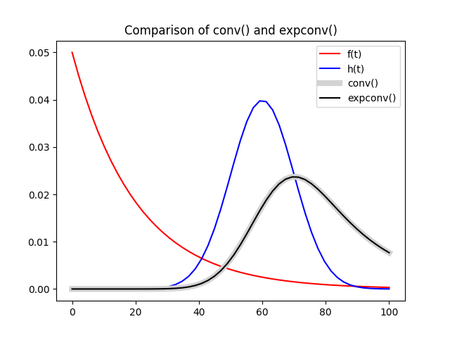
The result shows that the difference in accuracy between expconv and conv is negligible at higher time resolution. However, expconv comes with a major improvement in computation time. We illustrate the effect by applying the functions 500 times and measuring the total computation time in each case:

# Print the duration of 500 runs of conv:
start = time.time()
for _ in range(500):
    dc.conv(h, f, t)
print('Computation time for conv(): ', time.time()-start, 'sec')

# Print the duration of 500 runs of expconv:
start = time.time()
for _ in range(500):
    dc.expconv(h, Tf, t)
print('Computation time for expconv(): ', time.time()-start, 'sec')

Computation time for conv():  1.1724777221679688 sec
Computation time for expconv():  0.03907656669616699 sec

The acceleration is 2 orders of magnitude. Incidentally since the time array in this case is uniform, conv can be accelerated by specifying dt instead of t in the arguments. However the performance remains far below expconv:

# Print the duration of 500 runs of conv with uniform dt:
start = time.time()
for i in range(500):
    dc.conv(h, f, dt=t[1])
print('Computation time for conv(): ',
      time.time()-start, 'sec')

Computation time for conv():  0.5115406513214111 sec

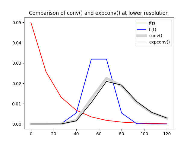
The difference in accuracy between conv and expconv becomes more apparent at lower temporal resolution but generally remains minor. Using 10 time points instead of 50 as above we start seeing some effect:

# Generate Gaussian and exponential at low temporal resolution:
t = np.linspace(0, 120, 10)
h = norm.pdf(t, 60, 10)
f = np.exp(-t/Tf)/Tf

# Convolve the Gaussian with the exponential in two different ways:
g0 = dc.conv(h, f, t)
g1 = dc.expconv(h, Tf, t)

# Compare the result on the same plot:
plt.plot(t, f, 'r-', label='f(t)')
plt.plot(t, h, 'b-', label='h(t)')
plt.plot(t, g0, label='conv()', linewidth=6, color='lightgray', linestyle='-')
plt.plot(t, g1, 'k-', label='expconv()')
plt.title('Comparison of conv() and expconv() at lower resolution')
plt.legend()
plt.show()

Convolving two or more exponentials

If both functions are exponentials, convolution can be accelerated further with biexpconv, which uses an analytical formula to calculate the convolution:

# Create and exponential dataset:
Th = 10
h = np.exp(-t/Th)/Th

# Print the duration of 1000 runs of expconv:
start = time.time()
for i in range(1000):
    dc.expconv(h, Tf, t)
print('Computation time for expconv(): ', time.time()-start, 'sec')

# Print the duration of 1000 runs of biexpconv:
start = time.time()
for i in range(1000):
    dc.biexpconv(Th, Tf, t)
print('Computation time for biexpconv(): ', time.time()-start, 'sec')

Computation time for expconv():  0.03711819648742676 sec
Computation time for biexpconv():  0.00797891616821289 sec

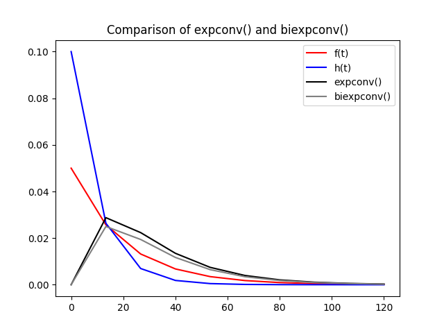
The difference in computation time is small in this case, but using an analytical formula also comes with some improvements in accuracy. This is apparent at lower time resolution:

# Compute a bioexponential convolution with expconv:
g0 = dc.expconv(h, Tf, t)

# Compute a biexponential convolution with biexpconv:
g1 = dc.biexpconv(Th, Tf, t)

# Compare the results on the same plot:
plt.plot(t, f, 'r-', label='f(t)')
plt.plot(t, h, 'b-', label='h(t)')
plt.plot(t, g0, 'k-', label='expconv()')
plt.plot(t, g1, color='gray', linestyle='-', label='biexpconv()')
plt.title('Comparison of expconv() and biexpconv()')
plt.legend()
plt.show()

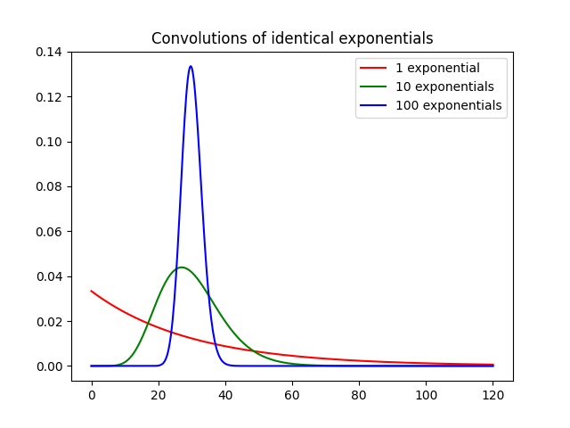
The final convolution function nexpconv convolves n indentical exponentials with mean transit time T analytically. We illustrate the result by keeping the total mean transit time MTT=nT constant, and increasing n from 1 to 100. As the number of exponentials increases, the convolution converges to a delta function positioned on t=MTT:

# Convolve 1, 10 and 100 indentical exponentials with the same total MTT:
MTT = 30
t = np.linspace(0, 120, 500)
g1 = dc.nexpconv(1, MTT/1, t)
g10 = dc.nexpconv(10, MTT/10, t)
g100 = dc.nexpconv(100, MTT/100, t)

# Compare the results on the same plot
plt.plot(t, g1, 'r-', label='1 exponential')
plt.plot(t, g10, 'g-', label='10 exponentials')
plt.plot(t, g100, 'b-', label='100 exponentials')
plt.title('Convolutions of identical exponentials')
plt.legend()
plt.show()

Convolution with a step function

dcmri also provides a dedicated function stepconv for convolution with a step function. We illustrate this function here and compare against conv:

# Generate some Gaussian data:
n = 15
t = np.linspace(0, 120, n)
f = norm.pdf(t, 30, 10)
T, D = 45, 0.5

# Construct a step function explicitly:
T0, T1 = T-D*T, T+D*T
h = np.zeros(n)
h[(t>=T0)*(t<=T1)] = 1/(T1-T0)

# Convolve the step function with the Gaussian using conv:
g0 = dc.conv(h, f, t)

# Convolve the step function with the Gaussian using stepconv:
g1 = dc.stepconv(f, T, D, t)

# Compare the results on the same plot:
plt.plot(t, f, 'r-', label='f(t)')
plt.plot(t, g0, 'k-', label='conv()')
plt.plot(t, g1, color='gray', linestyle='-', label='stepconv()')
plt.title('Comparison of conv() and stepconv()')
plt.legend()
plt.show()

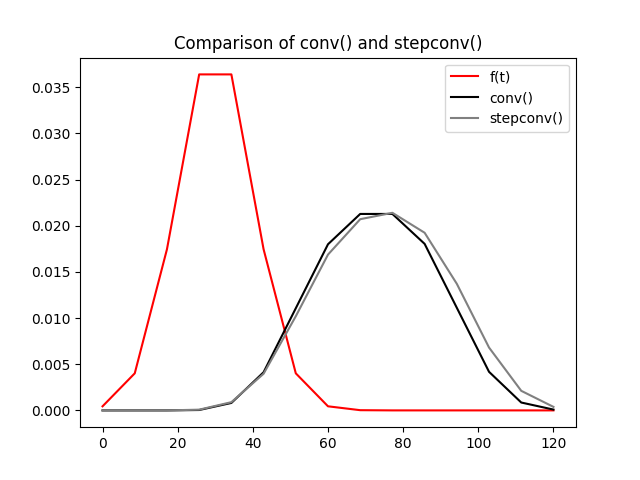
As with expconv the difference between stepconv and conv is relatively small even for coarse time grids such as the above, but there is a more substantial gain in computation time:

# Print the computation time for 500 runs of conv:
start = time.time()
for _ in range(500):
    dc.conv(h, f, t)
print('Computation time for conv(): ', time.time()-start, 'sec')

# Print the computation time for 500 runs of stepconv:
start = time.time()
for _ in range(500):
    dc.stepconv(f, T, D, t)
print('Computation time for stepconv(): ', time.time()-start, 'sec')

Computation time for conv():  0.4879117012023926 sec
Computation time for stepconv():  0.2529292106628418 sec