dcmri.TissueLSArray#

class dcmri.TissueLSArray(shape, sequence='SS', **kwargs)[source]#

Array of linear and stationary tissues with a single inlet.

These are generic model-free tissue types. Their response to an indicator injection is proportional to the dose (linear) and independent of the time of injection (stationary).

Parameters:

shape (array-like, required) – shape of the tissue array (spatial dimensions only). Any number of dimensions is allowed.
aif (array-like, required) – Signal-time curve in the blood of the feeding artery.
dt (float, optional) – Time interval between values of the arterial input function. Defaults to 1.0.
sequence (str, optional) – imaging sequence. Possible values are ‘SS’, ‘SR’ and ‘lin’ (linear). Defaults to ‘SS’.
params (dict, optional) – values for the parameters of the tissue, specified as keyword parameters. Defaults are used for any that are not provided.

See also

TissueLS, TissueArray

Example

Fit a linear and stationary model to the synthetic test images:

>>> import numpy as np
>>> import dcmri as dc

Use fake_brain to generate synthetic test data:

>>> n=64
>>> time, signal, aif, gt = dc.fake_brain(n)

The correct ground truth for ve in model-free analysis is the extracellular part of the distribution space:

>>> gt['ve'] = gt['ve'] = np.where(gt['PS'] > 0, gt['vp'] + gt['vi'], gt['vp'])

Build a tissue array and set the constants to match the experimental conditions of the synthetic test data. We use the exact T1-map as baseline values:

>>> tissue = dc.TissueLSArray(
...     (n,n),
...     dt = time[1],
...     sequence = 'SS',
...     r1 = dc.relaxivity(3, 'blood','gadodiamide'),
...     TR = 0.005,
...     FA = 15,
...     R10a = 1/dc.T1(3.0,'blood'),
...     R10 = np.where(gt['T1']==0, 0, 1/gt['T1']),
... )

Train the tissue on the data. Since have noise-free synthetic data we use a lower tolerance than the default, which is optimized for noisy data:

>>> tissue.train(signal, aif, n0=10, tol=0.01)

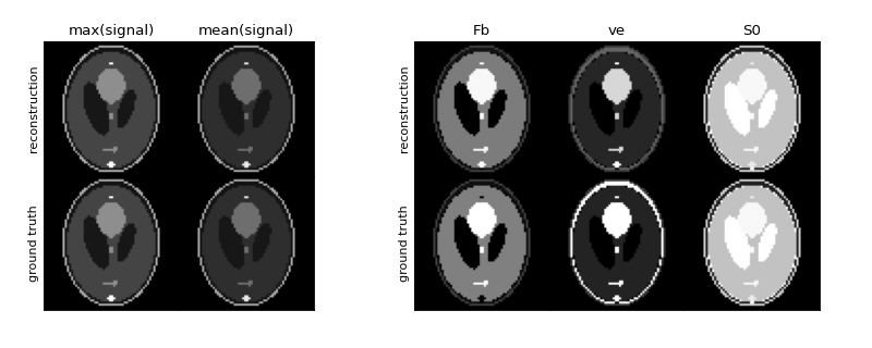
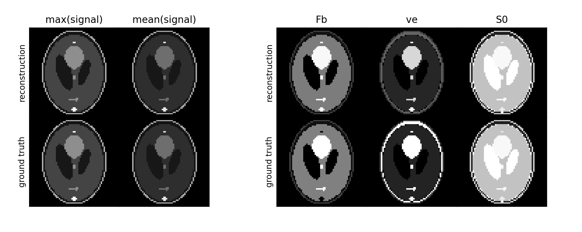
Plot the reconstructed maps, along with the ground truth for reference. We set fixed scaling for the parameter maps so they are comparable.

>>> vmin = {'Fb':0, 've':0, 'S0':0}
>>> vmax = {'Fb':0.02, 've':0.2, 'S0':np.amax(gt['S0'])}
>>> tissue.plot(vmin=vmin, vmax=vmax, ref=gt)

(Source code, png, hires.png, pdf)

Notes

As the example shows, even under noise-free conditions the maps are not reconstructed exactly. While the assumptions of linearity and stationarity are valid for the data generated by fake_brain, the price to pay for a fully model-free analysis is some numerical bias. The advantage is a convenient and fast first line analysis that applies under practically all conditions and produces robust maps that provide a quantitative insight into functional differences between tissue types.

Methods

`params`(*args)	Export the tissue parameters
`plot`([vmin, vmax, cmap, ref, fname, show])	Plot parameter maps (all on one image)
`plot_overlay`([mask, vmin, vmax, ...])	Plot parameter maps (one image per parameter)
`predict`()	Predict the signal at specific time points
`predict_aif`()	Predict the signal at specific time points
`predict_conc`()	Return the tissue concentration
`train`(signal, signal_aif[, n0, tol, init_s0])	Train the free parameters

params(*args)[source]#

Export the tissue parameters

Parameters:: args (tuple) – parameters to get. If no arguments are provided, all available parameters are returned.
Returns:: Dictionary with tissue parameters.
Return type:: dict

plot(vmin={}, vmax={}, cmap='gray', ref=None, fname=None, show=True)[source]#

Plot parameter maps (all on one image)

Note: this function is currently only available for 2D data.

Parameters:

vmin (dict, optional) – Minimum values on display for given parameters. Defaults to {}.
vmax (dict, optional) – Maximum values on display for given parameters. Defaults to {}.
cmap (str, optional) – matplotlib colormap. Defaults to ‘gray’.
ref (dict, optional) – Reference images - typically used to display ground truth data when available. Keys are ‘signal’ (array of data in the same shape as signal), and the parameter maps to show. Defaults to None.
fname (str, optional) – File path to save image. Defaults to None.
show (bool, optional) – Determine whether the image is shown or not. Defaults to True.

Raises:

NotImplementedError – Features that are not currently implemented.

plot_overlay(mask=None, vmin=None, vmax=None, aspect_ratio=1.7777777777777777, cmap='magma', fname=None, show=True)[source]#

Plot parameter maps (one image per parameter)

Note: this function is currently only available for 3D data.

Parameters:

signal (numpy.ndarray) – dynamic signal
mask (numpy.ndarray) – If provided, only pixels inside the mask are shown
vmin (dict, optional) – Minimum values on display for the model parameters. Defaults to None.
vmax (dict, optional) – Maximum values on display for the model parameters. Defaults to None.
aspect_ratio (float, optional) – Aspect ratio of the mosaic. Defaults to 16/9.
cmap (str, optional) – matplotlib colormap. Defaults to ‘gray’.
fname (str, optional) – File path to save image. Defaults to None.
show (bool, optional) – Determine whether the image is shown or not. Defaults to True.

Raises:

NotImplementedError – Features that are not currently implemented.

predict()[source]#

Predict the signal at specific time points

Returns:: Array of predicted signals for each time point.
Return type:: np.ndarray

predict_aif()[source]#

Predict the signal at specific time points

Returns:: Array of predicted signals for each time point.
Return type:: np.ndarray

predict_conc()[source]#

Return the tissue concentration

Returns:: Concentration in M
Return type:: np.ndarray

train(signal, signal_aif, n0=1, tol=0.1, init_s0=True)[source]#

Train the free parameters

Parameters:

signal (array-like) – Array with measured signals.
tol – cut-off value for the singular values in the computation of the matrix pseudo-inverse.

Returns:

self

dcmri.TissueLSArray#

This Page