dcmri.TissueLS#

class dcmri.TissueLS(sequence='SS', **kwargs)[source]#

Array of linear and stationary tissues with a single inlet.

These are generic model-free tissue types. Their response to an indicator injection is proportional to the dose (linear) and independent of the time of injection (stationary).

Parameters:

shape (array-like, required) – shape of the tissue array (spatial dimensions only). Any number of dimensions is allowed.
aif (array-like, required) – Signal-time curve in the blood of the feeding artery.
dt (float, optional) – Time interval between values of the arterial input function. Defaults to 1.0.
sequence (str, optional) – imaging sequence. Possible values are ‘SS’, ‘SR’ and ‘lin’ (linear). Defaults to ‘SS’.
params (dict, optional) – values for the parameters of the tissue, specified as keyword parameters. Defaults are used for any that are not provided.

See also

TissueLS, TissueArray

Example

Fit a linear and stationary model to the synthetic test data:

>>> import numpy as np
>>> import dcmri as dc

Generate synthetic test data:

>>> time, aif, roi, gt = dc.fake_tissue()

The correct ground truth for ve in model-free analysis is the extracellular part of the distribution space:

>>> gt['ve'] = gt['vp'] + gt['vi'] if gt['PS'] > 0 else gt['vp']

Build a tissue and set the constants to match the experimental conditions of the synthetic test data.

>>> tissue = dc.TissueLS(
...     dt = time[1],
...     sequence = 'SS',
...     r1 = dc.relaxivity(3, 'blood','gadodiamide'),
...     TR = 0.005,
...     FA = 15,
...     R10a = 1/dc.T1(3.0,'blood'),
...     R10 = 1/dc.T1(3.0,'muscle'),
... )

Train the tissue on the data. Since have noise-free synthetic data we use a lower tolerance than the default, which is optimized for noisy data:

>>> tissue.train(roi, aif, n0=10, tol=0.01)

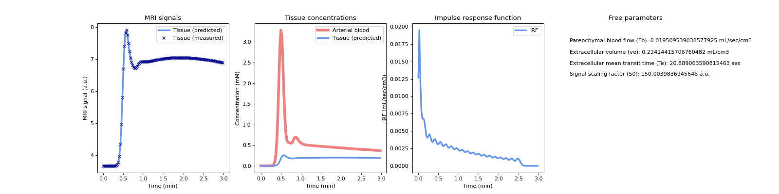
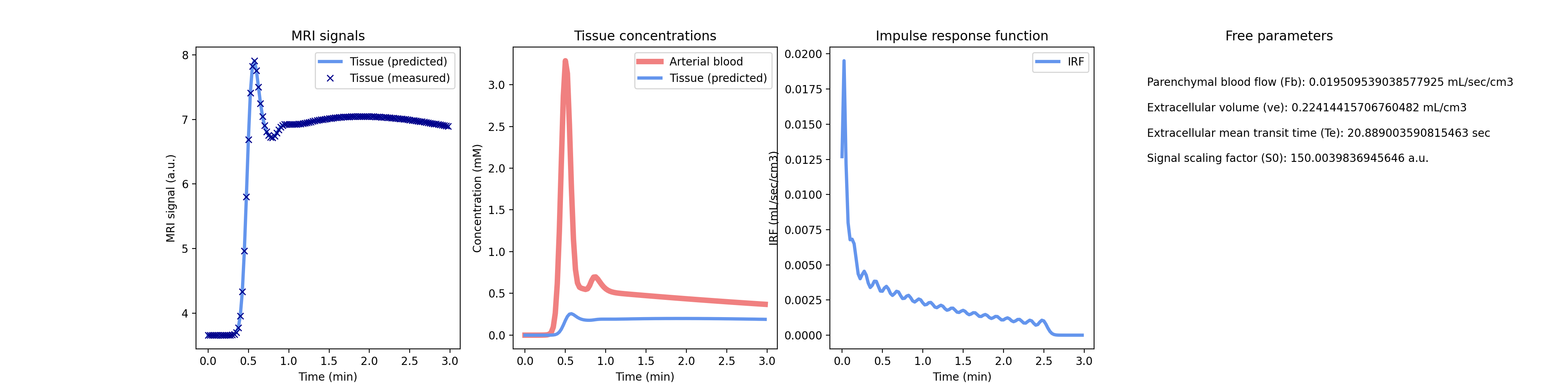
Plot the reconstructed signals along with the concentrations and the impulse response function.

>>> tissue.plot(roi)

(Source code, png, hires.png, pdf)

Methods

`params`(*args)	Export the tissue parameters
`plot`([signal, round_to, fname, show])	Plot the model fit against data
`predict`()	Predict the signal at specific time points
`predict_aif`()	Predict the signal at specific time points
`predict_conc`()	Return the tissue concentration
`print_params`([round_to])	Print the model parameters
`train`(signal, signal_aif[, n0, tol, init_s0])	Train the free parameters

params(*args)[source]#

Export the tissue parameters

Parameters:: args (tuple) – parameters to get. If no arguments are provided, all available parameters are returned.
Returns:: Dictionary with tissue parameters.
Return type:: dict

plot(signal=None, round_to=None, fname=None, show=True)[source]#

Plot the model fit against data

Parameters:

signal (array-like, optional) – Array with measured signals.
round_to (int, optional) – Rounding for the model parameters.
fname (path, optional) – Filepath to save the image. If no value is provided, the image is not saved. Defaults to None.
show (bool, optional) – If True, the plot is shown. Defaults to True.

predict()[source]#

Predict the signal at specific time points

Returns:: Array of predicted signals for each time point.
Return type:: np.ndarray

predict_aif()[source]#

Predict the signal at specific time points

Returns:: Array of predicted signals for each time point.
Return type:: np.ndarray

predict_conc()[source]#

Return the tissue concentration

Returns:: Concentration in M
Return type:: np.ndarray

print_params(round_to=None)[source]#

Print the model parameters

Parameters:: round_to (int, optional) – Round to how many digits. If this is not provided, the values are not rounded. Defaults to None.

train(signal, signal_aif, n0=1, tol=0.1, init_s0=True)[source]#

Train the free parameters

Parameters:

signal (array-like) – Array with measured signals.
tol – cut-off value for the singular values in the computation of the matrix pseudo-inverse.

Returns:

self

dcmri.TissueLS#

This Page