dcmri.conc_src

dcmri.conc_src(S, TC, T10, r1=0.005, n0=1, S0=None)

Concentration of a saturation-recovery sequence with a center-encoded readout.

Parameters:

• S (array-like) – Signal in arbitrary units.

• TC (float) – Time (sec) between the saturation pulse and the acquisition of the k-space center.

• T10 (float) – baseline T1 value in sec.

• r1 (float, optional) – Longitudinal relaxivity in Hz/M. Defaults to 0.005.

• n0 (int, optional) – Baseline length. Defaults to 1.

Returns:

Concentration in M, same length as S.

Return type:

np.ndarray

Example

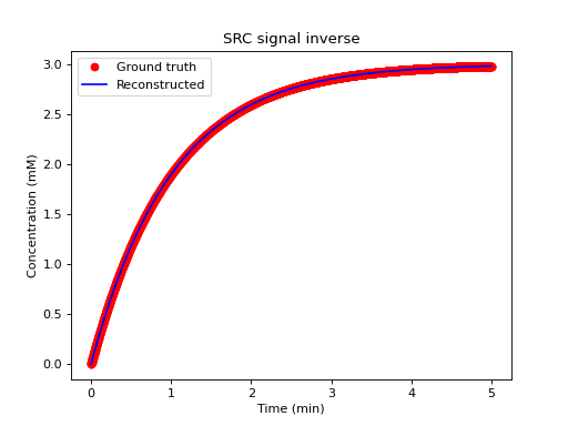
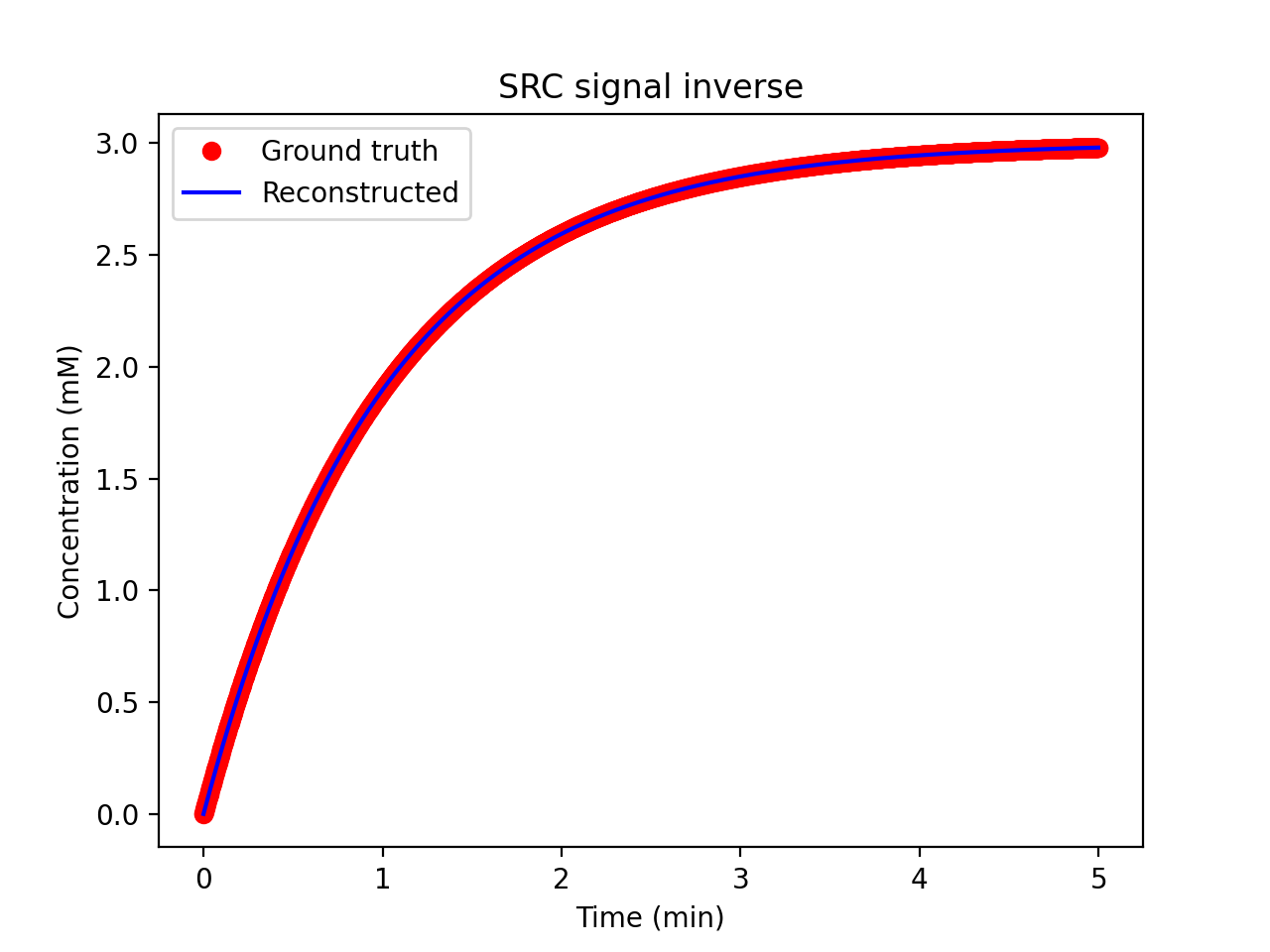
We generate some signals from ground-truth concentrations, then reconstruct the concentrations and check against the ground truth:

>>> import matplotlib.pyplot as plt
>>> import numpy as np
>>> import dcmri as dc

First define some constants:

>>> T10 = 1         # sec
>>> TC = 0.2        # sec
>>> r1 = 0.005      # Hz/M
>>> FA = 15         # deg

Generate ground truth concentrations and signal data:

>>> t = np.arange(0, 5*60, 0.1)     # sec
>>> C = 0.003*(1-np.exp(-t/60))     # M
>>> R1 = 1/T10 + r1*C               # Hz
>>> S = dc.signal_free(100, R1, TC, FA)  # au

Reconstruct the concentrations from the signal data:

>>> Crec = dc.conc_src(S, TC, T10, r1)

Check results by plotting ground truth against reconstruction:

>>> plt.plot(t/60, 1000*C, 'ro', label='Ground truth')
>>> plt.plot(t/60, 1000*Crec, 'b-', label='Reconstructed')
>>> plt.title('SRC signal inverse')
>>> plt.xlabel('Time (min)')
>>> plt.ylabel('Concentration (mM)')
>>> plt.legend()
>>> plt.show()

(Source code, png, hires.png, pdf)