dcmri.Mz_free#
- dcmri.Mz_free(R1, T, v=1, Fw=0, j=None, n0=0, me=1)[source]#
Free longitudinal magnetization.
See section Longitudinal relaxation for more detail.
- Parameters:
R1 (array-like) – Longitudinal relaxation rates in 1/sec. For a tissue with n compartments, the first dimension of R1 must be n. For a single compartment, R1 can be scalar or a 1D time-array.
T (array-like) – duration of free recovery.
v (array-like, optional) – volume fractions of the compartments. For a one-compartment tissue this is a scalar - otherwise it is an array with one value for each compartment. Defaults to 1.
Fw (array-like, optional) – Water flow between the compartments and to the environment, in units of mL/sec/cm3. Generally Fw must be a nxn array, where n is the number of compartments, and the off-diagonal elements Fw[j,i] are the permeability for water moving from compartment i into j. The diagonal elements Fw[i,i] quantify the flow of water from compartment i to outside. For a closed system with equal permeabilities between all compartments, a scalar value for Fw can be provided. Defaults to 0.
j (array-like, optional) – normalized tissue magnetization flux. j has to have the same shape as R1. Defaults to None.
n0 (array-like, optional) – initial relative magnetization at T=0. If this is a scalar, all compartments are assumed to have the same initial magnetization. Defaults to 0.
me (array-like, optional) – equilibrium magnetization of the tissue compartments. If a scalar value is provided, all compartments are assumed to have the same equilibrium magnetization. Defaults to 1.
- Returns:
Magnetization in the compartments after a time T.
- Return type:
np.ndarray
Example
Magnetization recovery after inversion.
>>> import numpy as np
>>> import matplotlib.pyplot as plt
>>> import dcmri as dc
Plot magnetization recovery for the first 10 seconds after an inversion pulse, for a closed tissue with R1 = 1 sec, and for an open tissue with equilibrium inflow and inverted inflow:
>>> TI = 0.1*np.arange(100)
>>> R1 = 1
>>> f = 0.5
>>> Mz = dc.Mz_free(R1, TI, n0=-1)
>>> Mz_e = dc.Mz_free(R1, TI, n0=-1, Fw=f, j=f)
>>> Mz_i = dc.Mz_free(R1, TI, n0=-1, Fw=f, j=-f)
>>> plt.plot(TI, Mz, label='No flow', linewidth=3)
>>> plt.plot(TI, Mz_e, label='Equilibrium inflow', linewidth=3)
>>> plt.plot(TI, Mz_i, label='Inverted inflow', linewidth=3)
>>> plt.xlabel('Inversion time (sec)')
>>> plt.ylabel('Magnetization (A/cm)')
>>> plt.legend()
>>> plt.show()
(
Source code,png,hires.png,pdf)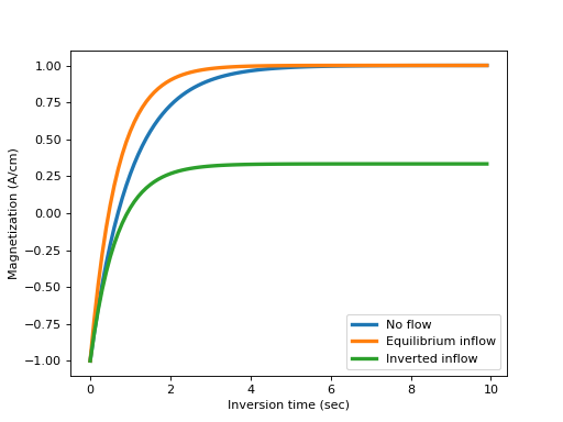
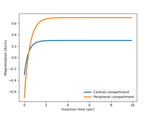
Now consider a two-compartment model, with a central compartment that has in- and outflow, and a peripheral compartment that only exchanges with the central compartment:
>>> R1 = [1,2]
>>> v = [0.3, 0.7]
>>> PS = 0.1
>>> Fw = [[f, PS], [PS, 0]]
>>> Mz = dc.Mz_free(R1, TI, v, Fw, n0=-1, j=[f, 0])
>>> plt.plot(TI, Mz[0,:], label='Central compartment', linewidth=3)
>>> plt.plot(TI, Mz[1,:], label='Peripheral compartment', linewidth=3)
>>> plt.xlabel('Inversion time (sec)')
>>> plt.ylabel('Magnetization (A/cm)')
>>> plt.legend()
>>> plt.show()

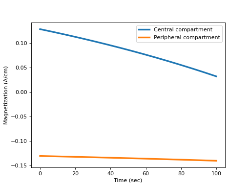
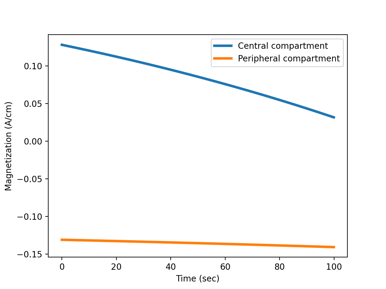
In DC-MRI the more usual situation is one where TI is fixed and the relaxation rates are variable due to the effect of a contrast agent. As an illustration, consider the previous result again at TI=500 msec and an R1 that is linearly declining in the central compartment and constant in the peripheral compartment:
>>> TI = 0.5
>>> nt = 1000
>>> t = 0.1*np.arange(nt)
>>> R1 = np.stack((1-t/np.amax(t), np.ones(nt)))
>>> j = np.stack((f*np.ones(nt), np.zeros(nt)))
>>> Mz = dc.Mz_free(R1, TI, v, Fw, n0=-1, j=j)
>>> plt.plot(t, Mz[0,:], label='Central compartment', linewidth=3)
>>> plt.plot(t, Mz[1,:], label='Peripheral compartment', linewidth=3)
>>> plt.xlabel('Time (sec)')
>>> plt.ylabel('Magnetization (A/cm)')
>>> plt.legend()
>>> plt.show()

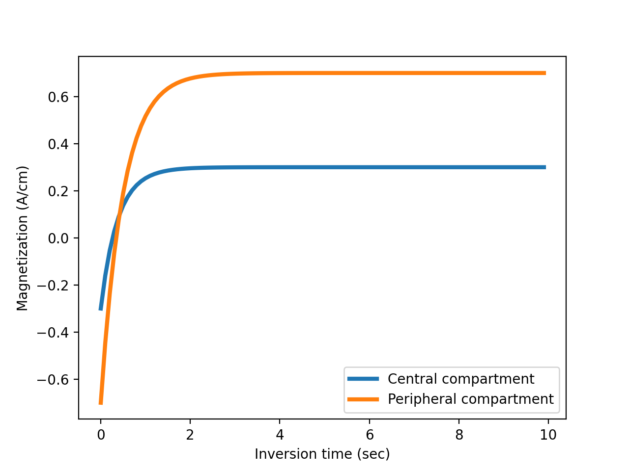
The function allows for R1 and TI to be both variable. Computing the result for 10 different TI values and extracting the result corresponding to TI=0.5 gives again the same result:
>>> TI = 0.1*np.arange(10)
>>> Mz = dc.Mz_free(R1, TI, v, Fw, n0=-1, j=j)
>>> plt.plot(t, Mz[0,:,5], label='Central compartment', linewidth=3)
>>> plt.plot(t, Mz[1,:,5], label='Peripheral compartment', linewidth=3)
>>> plt.xlabel('Time (sec)')
>>> plt.ylabel('Magnetization (A/cm)')
>>> plt.legend()
>>> plt.show()
